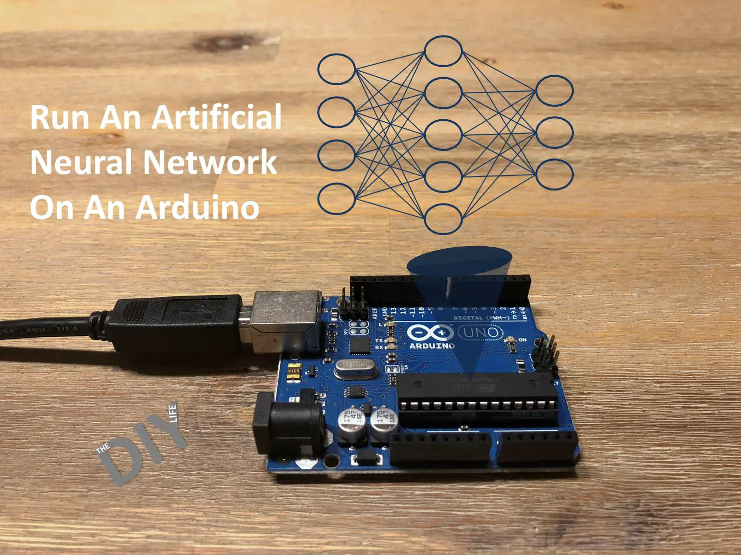
(AI)-XOR Function and Its Interpretation through Artificial Neural Networks
Historical Importance
The XOR problem gained historical significance in the late 1960s when it was presented as a critique of the perceptron model by Marvin Minsky and Seymour Papert. Their work demonstrated that single-layer perceptrons, which were prevalent at the time, could not solve simple non-linear problems like XOR. This discovery led to a significant setback in neural network research and contributed to the first AI winter, a period during which funding and interest in AI research dramatically decreased.
XOR Function
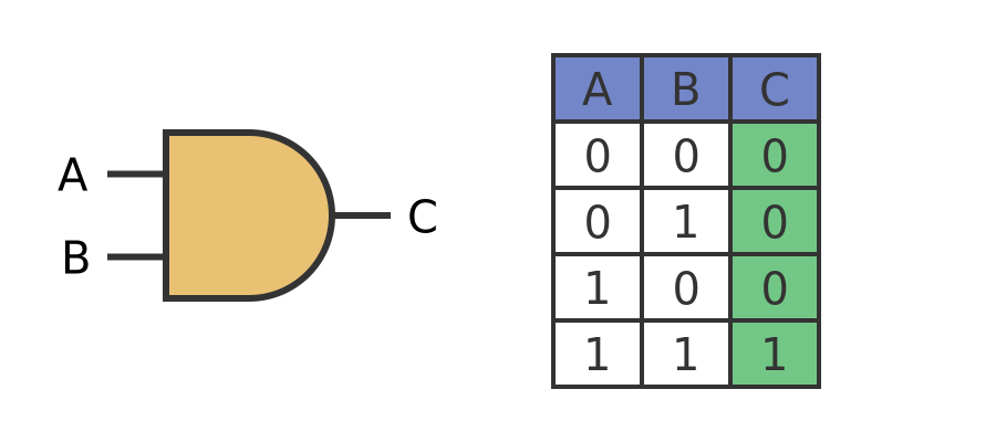
The XOR function, short for "exclusive or," is a type of logical operation that is fundamental to various fields of computing and digital electronics. XOR operates on two boolean inputs and produces a true value if, and only if, the inputs are different. If both inputs are the same, whether true or true or false or false, the XOR operation produces a false value. In terms of binary values, where true is represented as 1 and false as 0, the XOR operation can be summarized as follows:
Understanding Training in Artificial Neural Networks and Building a Three-Layer Feed forward Network
In this example, we'll construct a three-layer feed forward network consisting of an input layer, a hidden layer, and an output layer, as depicted below:

In this scenario, we have inputs representing the segments of an LED display and corresponding outputs showing their binary numbers. The network adjusts its settings as it repeatedly processes the training data until it reaches a satisfactory level of accuracy. At that point, we consider the network to be trained.

To track the training progress and view the final results, open the Serial Monitor in your Arduino IDE. The program will transmit a set of training data every one thousand cycles, allowing you to observe how the network is gradually improving and approaching the correct answers.
If you wish to train your network with custom data, refer to the last sections of this guide for instructions on creating your own training data.
Uploading code to an Arduino and observing the results through the Serial monitor is a great way to learn and understand how the code works, especially for projects like training a neural network.
Here is the code:
//Author: Ralph Heymsfeld
//28/06/2018

#include <math.h>

/******************************************************************
 * Network Configuration - customized per network
 ******************************************************************/

const int PatternCount = 10;
const int InputNodes = 7;
const int HiddenNodes = 8;
const int OutputNodes = 4;
const float LearningRate = 0.3;
const float Momentum = 0.9;
const float InitialWeightMax = 0.5;
const float Success = 0.0004;

const byte Input[PatternCount][InputNodes] = {
  { 1, 1, 1, 1, 1, 1, 0 },  // 0
  { 0, 1, 1, 0, 0, 0, 0 },  // 1
  { 1, 1, 0, 1, 1, 0, 1 },  // 2
  { 1, 1, 1, 1, 0, 0, 1 },  // 3
  { 0, 1, 1, 0, 0, 1, 1 },  // 4
  { 1, 0, 1, 1, 0, 1, 1 },  // 5
  { 0, 0, 1, 1, 1, 1, 1 },  // 6
  { 1, 1, 1, 0, 0, 0, 0 },  // 7
  { 1, 1, 1, 1, 1, 1, 1 },  // 8
  { 1, 1, 1, 0, 0, 1, 1 }   // 9
};

const byte Target[PatternCount][OutputNodes] = {
  { 0, 0, 0, 0 },
  { 0, 0, 0, 1 },
  { 0, 0, 1, 0 },
  { 0, 0, 1, 1 },
  { 0, 1, 0, 0 },
  { 0, 1, 0, 1 },
  { 0, 1, 1, 0 },
  { 0, 1, 1, 1 },
  { 1, 0, 0, 0 },
  { 1, 0, 0, 1 }
};

/******************************************************************
 * End Network Configuration
 ******************************************************************/


int i, j, p, q, r;
int ReportEvery1000;
int RandomizedIndex[PatternCount];
long  TrainingCycle;
float Rando;
float Error;
float Accum;


float Hidden[HiddenNodes];
float Output[OutputNodes];
float HiddenWeights[InputNodes+1][HiddenNodes];
float OutputWeights[HiddenNodes+1][OutputNodes];
float HiddenDelta[HiddenNodes];
float OutputDelta[OutputNodes];
float ChangeHiddenWeights[InputNodes+1][HiddenNodes];
float ChangeOutputWeights[HiddenNodes+1][OutputNodes];

void setup(){
  Serial.begin(9600);
  randomSeed(analogRead(3));
  ReportEvery1000 = 1;
  for( p = 0 ; p < PatternCount ; p++ ) {
    RandomizedIndex[p] = p ;
  }
}

void loop (){


/******************************************************************
* Initialize HiddenWeights and ChangeHiddenWeights
******************************************************************/

  for( i = 0 ; i < HiddenNodes ; i++ ) {
    for( j = 0 ; j <= InputNodes ; j++ ) {
      ChangeHiddenWeights[j][i] = 0.0 ;
      Rando = float(random(100))/100;
      HiddenWeights[j][i] = 2.0 * ( Rando - 0.5 ) * InitialWeightMax ;
    }
  }
/******************************************************************
* Initialize OutputWeights and ChangeOutputWeights
******************************************************************/

  for( i = 0 ; i < OutputNodes ; i ++ ) {
    for( j = 0 ; j <= HiddenNodes ; j++ ) {
      ChangeOutputWeights[j][i] = 0.0 ;
      Rando = float(random(100))/100;
      OutputWeights[j][i] = 2.0 * ( Rando - 0.5 ) * InitialWeightMax ;
    }
  }
  Serial.println("Initial/Untrained Outputs: ");
  toTerminal();
/******************************************************************
* Begin training
******************************************************************/

  for( TrainingCycle = 1 ; TrainingCycle < 2147483647 ; TrainingCycle++) {

/******************************************************************
* Randomize order of training patterns
******************************************************************/

    for( p = 0 ; p < PatternCount ; p++) {
      q = random(PatternCount);
      r = RandomizedIndex[p] ;
      RandomizedIndex[p] = RandomizedIndex[q] ;
      RandomizedIndex[q] = r ;
    }
    Error = 0.0 ;
/******************************************************************
* Cycle through each training pattern in the randomized order
******************************************************************/
    for( q = 0 ; q < PatternCount ; q++ ) {
      p = RandomizedIndex[q];

/******************************************************************
* Compute hidden layer activations
******************************************************************/

      for( i = 0 ; i < HiddenNodes ; i++ ) {
        Accum = HiddenWeights[InputNodes][i] ;
        for( j = 0 ; j < InputNodes ; j++ ) {
          Accum += Input[p][j] * HiddenWeights[j][i] ;
        }
        Hidden[i] = 1.0/(1.0 + exp(-Accum)) ;
      }

/******************************************************************
* Compute output layer activations and calculate errors
******************************************************************/

      for( i = 0 ; i < OutputNodes ; i++ ) {
        Accum = OutputWeights[HiddenNodes][i] ;
        for( j = 0 ; j < HiddenNodes ; j++ ) {
          Accum += Hidden[j] * OutputWeights[j][i] ;
        }
        Output[i] = 1.0/(1.0 + exp(-Accum)) ;
        OutputDelta[i] = (Target[p][i] - Output[i]) * Output[i] * (1.0 - Output[i]) ;
        Error += 0.5 * (Target[p][i] - Output[i]) * (Target[p][i] - Output[i]) ;
      }

/******************************************************************
* Backpropagate errors to hidden layer
******************************************************************/

      for( i = 0 ; i < HiddenNodes ; i++ ) {
        Accum = 0.0 ;
        for( j = 0 ; j < OutputNodes ; j++ ) {
          Accum += OutputWeights[i][j] * OutputDelta[j] ;
        }
        HiddenDelta[i] = Accum * Hidden[i] * (1.0 - Hidden[i]) ;
      }


/******************************************************************
* Update Inner-->Hidden Weights
******************************************************************/


      for( i = 0 ; i < HiddenNodes ; i++ ) {
        ChangeHiddenWeights[InputNodes][i] = LearningRate * HiddenDelta[i] + Momentum * ChangeHiddenWeights[InputNodes][i] ;
        HiddenWeights[InputNodes][i] += ChangeHiddenWeights[InputNodes][i] ;
        for( j = 0 ; j < InputNodes ; j++ ) {
          ChangeHiddenWeights[j][i] = LearningRate * Input[p][j] * HiddenDelta[i] + Momentum * ChangeHiddenWeights[j][i];
          HiddenWeights[j][i] += ChangeHiddenWeights[j][i] ;
        }
      }

/******************************************************************
* Update Hidden-->Output Weights
******************************************************************/

      for( i = 0 ; i < OutputNodes ; i ++ ) {
        ChangeOutputWeights[HiddenNodes][i] = LearningRate * OutputDelta[i] + Momentum * ChangeOutputWeights[HiddenNodes][i] ;
        OutputWeights[HiddenNodes][i] += ChangeOutputWeights[HiddenNodes][i] ;
        for( j = 0 ; j < HiddenNodes ; j++ ) {
          ChangeOutputWeights[j][i] = LearningRate * Hidden[j] * OutputDelta[i] + Momentum * ChangeOutputWeights[j][i] ;
          OutputWeights[j][i] += ChangeOutputWeights[j][i] ;
        }
      }
    }

/******************************************************************
* Every 1000 cycles send data to terminal for display
******************************************************************/
    ReportEvery1000 = ReportEvery1000 - 1;
    if (ReportEvery1000 == 0)
    {
      Serial.println();
      Serial.println();
      Serial.print ("TrainingCycle: ");
      Serial.print (TrainingCycle);
      Serial.print ("  Error = ");
      Serial.println (Error, 5);

      toTerminal();

      if (TrainingCycle==1)
      {
        ReportEvery1000 = 999;
      }
      else
      {
        ReportEvery1000 = 1000;
      }
    }


/******************************************************************
* If error rate is less than pre-determined threshold then end
******************************************************************/

    if( Error < Success ) break ;
  }
  Serial.println ();
  Serial.println();
  Serial.print ("TrainingCycle: ");
  Serial.print (TrainingCycle);
  Serial.print ("  Error = ");
  Serial.println (Error, 5);

  toTerminal();

  Serial.println ();
  Serial.println ();
  Serial.println ("Training Set Solved! ");
  Serial.println ("--------");
  Serial.println ();
  Serial.println ();
  ReportEvery1000 = 1;
}

void toTerminal()
{

  for( p = 0 ; p < PatternCount ; p++ ) {
    Serial.println();
    Serial.print ("  Training Pattern: ");
    Serial.println (p);
    Serial.print ("  Input ");
    for( i = 0 ; i < InputNodes ; i++ ) {
      Serial.print (Input[p][i], DEC);
      Serial.print (" ");
    }
    Serial.print ("  Target ");
    for( i = 0 ; i < OutputNodes ; i++ ) {
      Serial.print (Target[p][i], DEC);
      Serial.print (" ");
    }
/******************************************************************
* Compute hidden layer activations
******************************************************************/

    for( i = 0 ; i < HiddenNodes ; i++ ) {
      Accum = HiddenWeights[InputNodes][i] ;
      for( j = 0 ; j < InputNodes ; j++ ) {
        Accum += Input[p][j] * HiddenWeights[j][i] ;
      }
      Hidden[i] = 1.0/(1.0 + exp(-Accum)) ;
    }

/******************************************************************
* Compute output layer activations and calculate errors
******************************************************************/

    for( i = 0 ; i < OutputNodes ; i++ ) {
      Accum = OutputWeights[HiddenNodes][i] ;
      for( j = 0 ; j < HiddenNodes ; j++ ) {
        Accum += Hidden[j] * OutputWeights[j][i] ;
      }
      Output[i] = 1.0/(1.0 + exp(-Accum)) ;
    }
    Serial.print ("  Output ");
    for( i = 0 ; i < OutputNodes ; i++ ) {
      Serial.print (Output[i], 5);
      Serial.print (" ");
    }
  }


}
--------------------------------------------------------------------------------------------------------------------
Once the code has been successfully downloads
1. Preparing the Arduino IDE
First, make sure you have the Arduino IDE installed on your computer. If you haven't installed it yet, you can download it from the official Arduino website.
2. Connecting the Arduino
Connect your Arduino board to your computer using a USB cable. The board should power on automatically.
3. Opening the Arduino IDE
Launch the Arduino IDE. You'll use this environment to write your code, upload it to the Arduino board, and monitor the output.
4. Selecting Your Board
Before uploading the code, you need to select your Arduino board model:
- Go to Tools > Board and choose your Arduino board model from the list (e.g., Arduino Uno, Nano, Mega, etc.).
5. Selecting the Port
- Go to Tools > Port and select the COM port that your Arduino is connected to. If you're unsure which port to select, disconnect your Arduino and reconnect it to see which port appears.
6. Copying the Code
In the large text area of the IDE, write your code or copy and paste the neural network code intended for your project.
7. Uploading the Code
Click the Upload button (the right arrow icon) in the IDE. This compiles the code and uploads it to your Arduino board. The process may take a few seconds to a minute. When the upload is successful, you'll see a message in the IDE's console at the bottom of the window.
8. Opening the Serial Monitor
- After uploading, open the Serial Monitor by clicking on the magnifying glass icon in the upper right corner of the IDE or go to Tools > Serial Monitor.
- Make sure the baud rate in the Serial Monitor matches the baud rate specified in your code (e.g.,
Serial.begin(9600);).
9. Observing the Training Process
With the Serial Monitor open, you can observe the output of your Arduino as it runs through the training data. This is particularly useful for neural network projects to see how the model is learning and adjusting over time.


Why does the number of training cycles vary with each training session of a machine learning model?
The variability in the number of training cycles each time a machine learning model is trained, for all exercises, can be attributed to several key factors directly drawn from established principles and practices in the field of machine learning and artificial intelligence:
Random Initialization: The initial weights of the model are set randomly. This fundamental randomness means each training starts from a different point, potentially following different paths towards optimization, thus affecting the number of cycles needed for convergence.
Stochastic Processes: Many training algorithms, particularly stochastic gradient descent, operate on random subsets of data for each cycle. This randomness in the selection of data impacts the efficiency and path of learning, leading to variations in the training duration.
Adaptive Learning Rates: The learning rate might change dynamically during training to optimize the learning process. Since these adjustments are based on the model's performance and can vary from one training session to another, they contribute to differences in the number of training cycles required.
Data Shuffle and Order: The order in which training data is presented to the model can significantly affect learning efficiency. Shuffling the data differently for each training session introduces variability in how quickly the model can learn the underlying patterns, affecting the number of training cycles.
Early Stopping Criteria: Training often incorporates early stopping to prevent over fitting, halting training when performance on a validation set ceases to improve. The point at which this lack of improvement triggers can vary, influencing the total number of training cycles.
Regularization and Dropout: Techniques designed to improve model generalization, such as dropout, introduce further variability. Dropout randomly omits units from the neural network during training, which can alter the model's learning trajectory and hence the number of cycles required for optimal training.
Footnote
https://www.the-diy-life.com/running-an-artificial-neural-network-on-an-arduino-uno/
https://graphicmaths.com/img/computer-science/logic/logic-gates/and-gate.png
https://www.the-diy-life.com/wp-content/uploads/2018/06/Running-An-Artifical-Neural-Network-On-An-Arduino-Uno.jpg?ezimgfmt=ng%3Awebp%2Fngcb1
https://www.the-diy-life.com/wp-content/uploads/2018/06/3-Layer-Feed-Fordward-Neural-Network-768x691.jpg?ezimgfmt=ng:webp/ngcb1
https://www.the-diy-life.com/wp-content/uploads/2018/06/LCD-7-Segment-Display-To-Binary.jpg?ezimgfmt=ng:webp/ngcb1

Comments
Post a Comment